
Core Concepts
Ona is built around a set of architectural ideas that distinguish it from conventional monitoring or analytics platforms. This page explains those ideas in depth — not just what Ona does, but why the system is designed the way it is.
System 1: Continuous Asset Monitoring
In Thinking, Fast and Slow, psychologist Daniel Kahneman described two modes of human cognition. System 1 is automatic, fast, and always running — it processes incoming signals continuously without requiring deliberate effort. System 2 is slow, effortful, and selective — it engages only when System 1 surfaces something worth reasoning about carefully.
Ona’s monitoring architecture is built on the same division.
The System 1 layer is a learned world model — a compact neural network that runs continuously across every inverter in a fleet, evaluating each five-minute telemetry window. Rather than checking whether sensor readings cross fixed thresholds, the world model learns what normal looks like for each asset: the relationship between irradiance, temperature, voltage, output power, and state across the full diurnal cycle, weather conditions, and seasonal variation.
When physical behavior departs from the model’s learned expectations, prediction error spikes. That spike is the anomaly signal — a quantified measure of how surprised the model is by what just happened. This violation-of-expectation approach detects gradual degradation, context-dependent faults, and precursor signals that hard-coded threshold rules cannot see.
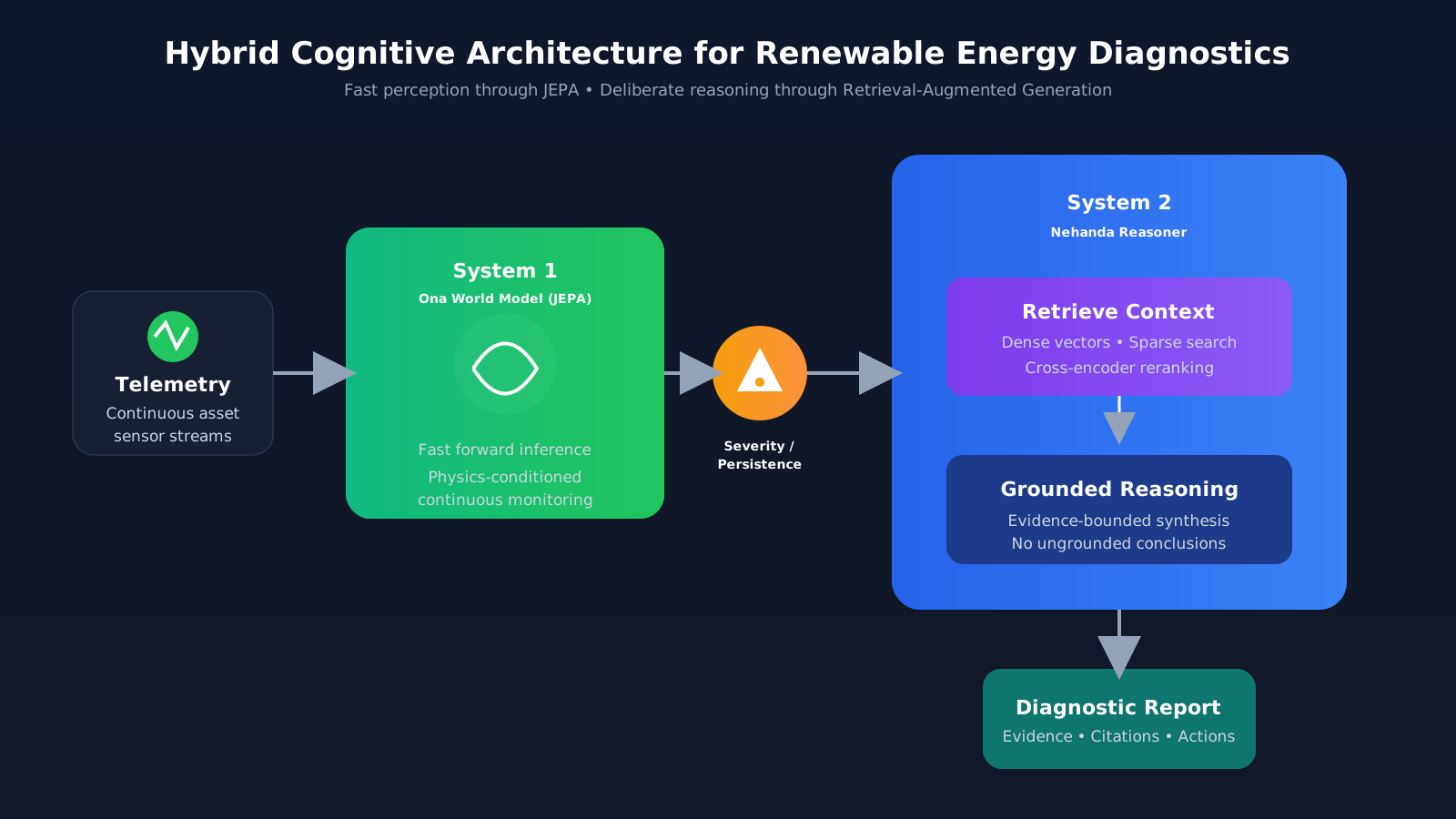
The diagram below maps this architecture: the world model runs cheaply on the left, gating access to the reasoner on the right. The threshold is not a tuning parameter — it is the economic and epistemic boundary between the two systems.
Why not just use threshold rules?
Traditional inverter monitoring relies on a small set of fixed conditions: run state equals zero, a fault code is present, output drops below a percentage of capacity. These rules work for obvious, discrete failures. They fail for:
- Gradual degradation — an inverter whose efficiency erodes over weeks without ever tripping a threshold
- Weather-conditional faults — low output that is perfectly normal given current cloud cover, or concerning given clear skies
- Novel failure modes — failure patterns that weren’t anticipated when the rules were written
- Early warning — precursor signals that appear before a fault code is ever generated
A learned world model captures the joint dynamics of normal operation. Any departure from that learned normal is anomalous, regardless of whether it matches a predefined rule.
What the world model does not do
The world model outputs a severity score. It does not explain why the score is elevated, identify the root cause, or recommend a corrective action. A score of 0.87 across six consecutive windows indicates that physical output has diverged significantly from the expected baseline — it does not distinguish between an overheating heat sink, a firmware handshake fault, or an isolated component failure buried inside a manufacturer troubleshooting guide.
That distinction is the work of System 2.
System 2: Diagnostic Synthesis
System 2 does not run continuously. It activates when System 1 outputs cross an explicit threshold — a severity score at or above a moderate level, or a sustained streak of anomalous windows. This gating is not an operational compromise. It is the architectural thesis.
Running a large language model on every five-minute telemetry packet would be prohibitively expensive and would eliminate the economic utility of the fast filter. The world model earns the compute cost of the reasoner. Cheap, narrow intelligence executes the vast majority of monitoring tasks; expensive, general intelligence is reserved for conditions that have earned it.
Retrieval-Augmented Generation
When System 2 activates, it does not rely on a language model’s memorized training knowledge to reason about the fault. Instead, it retrieves relevant content from a corpus of OEM manuals, field engineering guides, and maintenance documentation — tens of thousands of pages indexed for dense semantic search and sparse keyword matching.
Critically, the retrieval query is constructed automatically from the anomaly detection payload itself. Fault codes, power loss relative to an irradiance-conditioned baseline, component temperatures, and streak lengths are translated into the technical terminology used in manufacturer documentation. The anomaly writes its own question — there is no human writing a prompt.
This approach eliminates the main failure mode of unconstrained language model generation in industrial settings: confident, hallucinated repair instructions. If a model recommends a component replacement based on a fabricated failure mechanism, a field technician wastes a costly site visit. If the technician trusts the output and misses the real physical fault, the asset remains exposed to damage. Retrieval grounds the synthesis in verifiable sources. The model is trained to refuse explicitly when documentation is insufficient to establish cause.
Bounded intelligence as an operational requirement
The System 2 layer — Nehanda, a fine-tuned model running on Asoba’s own inference infrastructure — was optimized specifically for source fidelity and calibrated refusal, not for general capability. Domain-specific restraint outperforms parameter count for industrial diagnostic tasks. A model that confidently identifies the wrong cause is more dangerous than one that says “the available documentation does not establish a definitive cause for this failure pattern.”
The Decide and Act stages of the OODA loop remain entirely deterministic. The generative model does not dispatch technicians, execute switching commands, or alter physical control loops. Identical inputs yield identical control actions — a guarantee non-deterministic models cannot supply. Generative synthesis operates as an additive diagnostic field within the Orient phase, fully cited, confidence-bounded, and designed to surface uncertainty rather than paper over it.
Production Forecasting
Ona’s forecasting service produces device-, site-, and customer-level energy production forecasts. Understanding how forecasting works in Ona requires understanding why solar production forecasting is genuinely difficult, and what the architecture does to address that difficulty.
Why solar forecasting is hard
Solar production is not simply a function of current irradiance. It depends on the specific characteristics of each asset — the rated capacity, degradation history, inverter efficiency curve, and how the site responds to temperature and wind. It depends on weather conditions that change faster than most monitoring cycles. And it depends on time-of-day and seasonal irradiance geometry in ways that introduce strong periodicity that must be handled correctly to avoid autoregressive drift at night.
A naive model trained on one geography or one system type will generalize poorly. A model that ignores physics constraints will hallucinate production during nighttime hours. A model that cannot account for asset-specific behavior will produce fleet-average outputs that are individually meaningless.
How Ona addresses it
Ona’s forecasting models are trained to forecast production at multiple granularities using per-asset context, integrated weather data, and physics-informed constraints.
Asset-specific models are trained on each customer’s historical production data, enabling the model to learn the specific behavioral patterns of their fleet — not a generic proxy. Where sufficient customer history exists, the model adapts to actual site dynamics rather than population-level averages.
Weather integration is handled through a continuous weather cache that maintains live conditions and 48-hour ahead forecasts for every active deployment geography, updated at regular intervals. Irradiance, temperature, wind speed, cloud cover, and pressure are joined directly into the forecast input window, giving the model access to the same environmental signals that drive production.
Physics constraints are enforced during inference to preserve physical realism. Production is forced to zero when the Solar Zenith Angle exceeds 90° — the sun is below the horizon, and no model output should override that fact. Capacity normalization ensures that output predictions remain anchored to the actual installed capacity of the asset being forecast.
Autoregressive stability is maintained by keeping intermediate predictions in a normalized domain during multi-hour projection, then denormalizing only at the output boundary. This prevents the compounding error accumulation that can cause unconstrained autoregressive models to diverge over longer forecast horizons.
Freemium and customer-tailored models
Ona maintains two distinct model tiers. A generic baseline model, trained on a geographically diverse corpus of public solar datasets spanning multiple continents and climate zones, serves as the fallback for users without sufficient site-specific history. This model has broad coverage but is not optimized for any individual site.
Customer-tailored models are trained on a customer’s own production data once sufficient history has been collected. These models are materially more accurate for the specific sites they represent because they learn the actual behavioral signatures of those assets, not a population average.
The forecasting API resolves which model to use automatically — customer-tailored when available, generic baseline as fallback — without any configuration required from the caller.
Asset Intelligence
Ona computes a continuous set of asset health and financial metrics across every site, updated on an hourly schedule. These computations translate raw telemetry and anomaly data into the KPIs that matter for O&M decision-making:
Performance Ratio (PR) — the ratio of actual energy output to the theoretical output under measured irradiance conditions, following the IEC 61724 standard. PR quantifies how efficiently the system is converting available solar resource into delivered energy.
Availability — computed in three forms: 24/7 calendar availability, daytime-only availability, and energy-weighted availability (which reflects the fraction of available energy that was actually captured). Energy-weighted availability is the most operationally meaningful metric because a system that goes offline during peak irradiance hours causes disproportionate production loss.
Energy Achievement Ratio (EAR) — the gap between actual production and a contractual performance target, expressed in both energy (kWh) and financial terms. For SSEG installations, every kWh of shortfall below target is a kWh that must be replaced by grid power at full Time-of-Use tariff rates. The financial impact of underperformance is directly calculable.
Anomaly detection and maintenance signals — the asset intelligence layer identifies specific fault patterns across PV and battery assets, aggregates anomaly frequency over rolling windows, and generates forward-looking maintenance schedules. Assets exceeding an anomaly frequency threshold within a rolling 30-day window are flagged for inspection, with priority and recommended timing derived from the anomaly severity and manufacturer service interval data.
Battery State of Health (SOH) and warranty tracking — for fleets with Battery Energy Storage Systems (BESS), Ona tracks SOH, cycle count, depth of discharge patterns, and remaining warranted throughput against manufacturer warranty terms. Assets approaching warranty risk thresholds are surfaced before the window closes.
The OODA Loop
The OODA loop — Observe, Orient, Decide, Act — is a decision framework developed to describe how effective operators maintain situational awareness and respond to rapidly changing conditions. Ona is designed to close this loop end-to-end for distributed energy asset operations.
Observe: Five-minute telemetry from every inverter and battery asset flows continuously into the platform, normalized to a common schema regardless of manufacturer or device type.
Orient: The System 1 world model evaluates each telemetry window, scoring physical behavior against learned expectations. When a severity threshold is crossed, the System 2 retrieval and synthesis layer activates, retrieving relevant technical documentation and producing a cited diagnostic assessment. Asset intelligence computations translate aggregated telemetry into KPIs, anomaly signals, and financial impact estimates.
Decide: Maintenance schedules, work order priorities, and dispatch recommendations are generated from the orientation outputs. Decisions follow deterministic rules — they are not generated by the language model. Identical inputs always produce identical outputs.
Act: Maintenance workflows, work orders, BOM lookups, and job tracking close the loop from detection back to physical intervention, with activity feeds and issue tracking providing visibility across the entire O&M lifecycle.
The OODA loop is not metaphorical in Ona’s architecture. Each stage maps to specific services, each with defined inputs, outputs, and behavioral contracts. The SDK exposes this loop through typed clients that let operators and integrators interact with each stage programmatically.
For implementation details on any of the services described on this page, see the SDK Service Guides or the ODS-E & Architecture section.